Physics-based vision
Since I first got exposed to this topic - physics based vision, there is only one thing in my mind: it’s hard, and I hate it. Yet, I spent a lot of time reading textbooks, articles, papers, trying to understand the intuition and math. But this area is so vastly broad and after a while, the only recollection I had started to fade away. That’s why I decided to write this post, put down everything that I can or cannot understand.
From my own experience, the hardest part of this topic is the gap between the intuitiveness of the phenomena and the abstractness of the algorithms. It makes things even worse especially when you don’t implement every algorithm yourself.
The majority of the content is taken from the CPSC 505 course that I took in UBC (Courtesy to Prof. Bob Woodham and Prof. Jim Little), a CMU course Physics based Methods in Vision, and Computer Vision: a modern approach.
What is Physics-based vision
- How did the pixel get its value - Jitendra Malik
- We must understand scene appearance.
So what is scene appearance?
- Light and shadows
- Reflections
- Refractions
- Interreflections
- Scattering
Image Formation (Geometry)
Before we can estimate object/scene shape from images, we need to understand the geometric and radiometric relationship between the scene and its image.
Perspective Projection

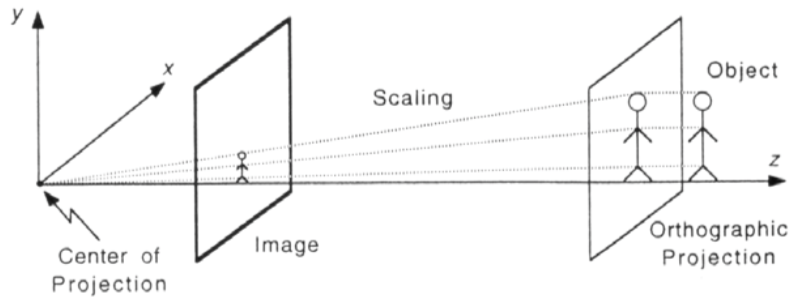
Orthographic Projection
This is only possible when \(z » \Delta z\), i.e., the range of scene depths is assumed to be much smaller than the average scene depth.

Better approximations to Perspective Projection
There are two alternative camera model that can better approximate perspective projection than orthographic projection: weak-perspective and para-perspective.
Weak-perspective: perspective projection onto a plane can be approximated by orthographic projection, followed by scaling, when (1) the object dimensions are small compared to the distance from the center of projection; (2) compared to this distance, the object is close to the optic axis.
Para-perspective: perspective projection onto a plane can be approximated by parallel projection, followed by scaling, whenever the object dimensions are small compared to the distance of the object from the center of projection. The direction of parallel projection is along the “average direction” of perspective projection. Parallel projection onto a plane is a generalisation of orthographic projection in which all the object points are projected along a set of parallel straight lines that may or may not be orthogonal to the image plane.
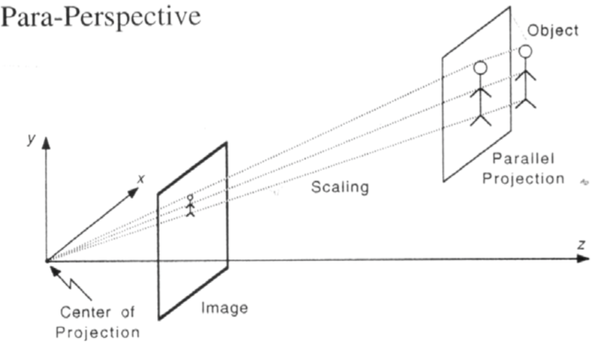
Image Formation (Radiometry)
We need to understand Radiometric Concepts and Reflectance Properties to interpret image intensities.
Image intensity
Image intensity is a function of illumination, surface reflectance and orientation, and surface reflection depends on both the viewing and illumination direction.
\[I = \int_A \int_{\Omega_i} \int_{\Omega_r} f(x, y, \omega_i, \omega_r) d\omega_i d\omega_r dA\]Radiometric concepts

- Solid angle: \(d\omega = \frac{dA’}{R^2}=\frac{dA cos\theta}{R^2}\) (steradian).
- Radiant Intensity of Source: \(J=\frac{d\Phi}{d\omega}\) (watts/steradian): Light Flux (power) emitted per unit solid angle.
-
Surface Irradiance: \(E=\frac{d\Phi}{dA}\) (watts/\(m^2\): Light Flux (power) incident per unit surface area. Does not depend on where the light is coming from.
- Inverse-square law: moving a point light source away from a surface reduces irradiance in proportion to the inverse square of the distance.
- Tilting a surface away from a point light results in a lower irradiance, in proportion to the cosine of the angle between the surface normal and the direction toward the light.
\[E(P) = \frac{1}{dA}L_i(P, \theta_i, \phi_i)(cos\theta_i dA)d\omega = L_i(P, \theta_i, \phi_i)cos\theta_i d\omega\]
- Surface Radiance: \(L = \frac{d^2\Phi}{(dAcos\theta_r)d\omega}\) (watts/\(m^2\) steradian), \(^2\) means there are 2 infinitesimal terms involved.
- Flux emitted per unit foreshortened/projected area per unit solid angle
- \(L\) depends on direction \(\theta_r\)
- Surface can radiate into whole hemisphere
- \(L\) depends on reflectance properties of surface
Radiance properties
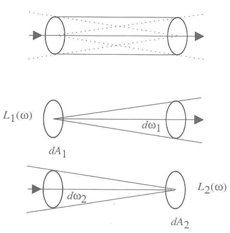
The distribution of light in space is a function of position and direction. The effect of illumination can be represented in terms of the power an infinitesimal patch of surface would receive if it were placed into space at a particular point and orientation. In other words, a small surface patch viewing the source frontally collects more evergy than the same patch viewing a source along a nearly tangent direction - the amoun of energy a patch collects from a source depends both on how large the source looks from the patch and on how large the patch looks from the source.
- Radiance is constant as it propagates along ray. More precisely, the radiance leaving \(P_1\) in the direction of \(P_2\) is the same as the radiance arriving \(P_2\) from the direction of \(P_1\).
Relation between scene and image brightness
Before lihgt hits the image plane (Linear Mapping):
\[\textit{Scene} \Rightarrow \textbf{Scene Radiance L} \Rightarrow \textit{Lens} \Rightarrow \textbf{Image Irradiance E}\]\[E = L\frac{pi}{4}(\frac{d}{f})^2cos\alpha^4\]
where \(L\) is the object/scene radiance, \(d\) is the lens diameter, \(f\) is the focal length, \(\alpha\) is the angle between the normal of the image plane and the direction from image point to center of lens. This relationship implies:
- The image irradiance is proportional to the object radiance
- The image irradiance is proportional to the area of the lens and inversely proportional to the distance between its center and the image plane.
- The image irradiance is proportional to \(cos^4\alpha\) and falls off as the light rays deviate from the optical axis
After light hits the image plane (Non-linear Mapping): \(\textbf{Image Irradiance E} \Rightarrow \textit{Camera Electronics} \Rightarrow \textbf{Measured Pixel Values, I}\)
Surface Model [2]
The following section is summarized from Chap 3 of the paper - Surface Reflection: Physical and Geometrical Perspectives.
The way in which light is reflected by a surface is dependent on, among other factors, the microscopic shape characteristics of the surface. A smooth surface may reflect incident light in a single direction, while a rough surface may scatter the light in various directions. We need prior knowledge of the microscopic surface irregularities, or a model of the surface to determine the reflection of incident light.
The possible surface models are divided into 2 categories: surface with exactly known profiles and surfaces with random irregularities. An exact profile may be determined by measuring the height at each point on the surface by means of a sensor such as the stylus profilometer. This method is cumbersome and impractical. Hence, it’s more reasonable to model the surface as a random process, where it is described by a statistical distribution of either its height above a certain mean level, or its slope w.r.t its mean (macroscopic) slope. The section only discusses these two statistical approaches.
Height Distribution Model
The height coordinate \(h\) of the surface is expressed as random function of the coordinates \(x\) and \(y\).
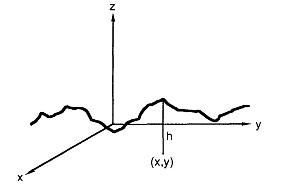
The shape of the surface is determined by the probability distribution of \(h\). For instance, let \(h\) be normally distributed, with mean value \(\bar{h}=0\) and standard deviation \(\sigma_h\). Then, the distribution of \(h\) is given by:
\[p_h(h)=\frac{1}{\sqrt{2\pi}\sigma_h}e^{-\frac{h^2}{2\sigma_h^2}}\]The \(\sigma_h\) is the root-mean-square of \(h\) and represents the roughness of the surface. The surface is not uniquely described by the distribution of \(h\), as it does not tell us anything about the distance between the hills and valleys of the surface.
The surfaces below have the same height distribution function, i.e., the same mean value and standard deviation. However, they don’t resemble each other in appearance.
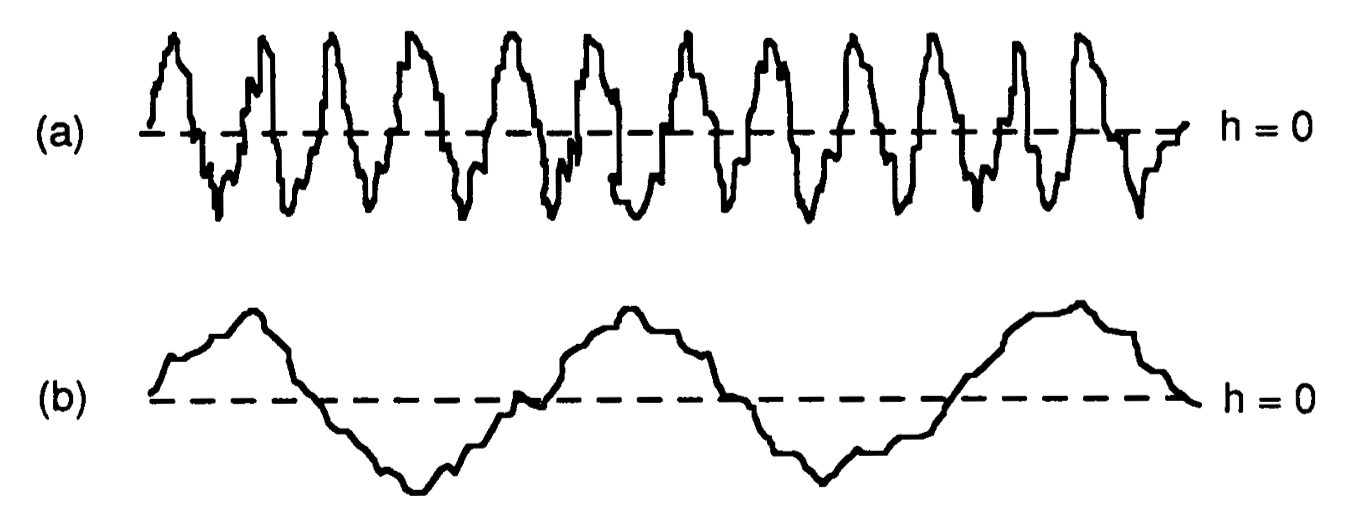
An autocorrelation coefficient \(C(\tau)\) is introduced, that determines the correlation (or lack of independence) between the random values assumed by the height \(h\) at two surface points \((x_1, y_1)\) and \((x_2, y_2)\), separated by a distance \(\tau\). The autocorrelation coefficient can be:
\[C(\tau)=e^{-\frac{\tau^2}{T^2}}\]where \(T\) is the correlation distance. Therefore, the above surfaces have small and large correlation distances respectively.
Slope Distribution Model
We can also think of a surface as a collection of planar micro-facets.
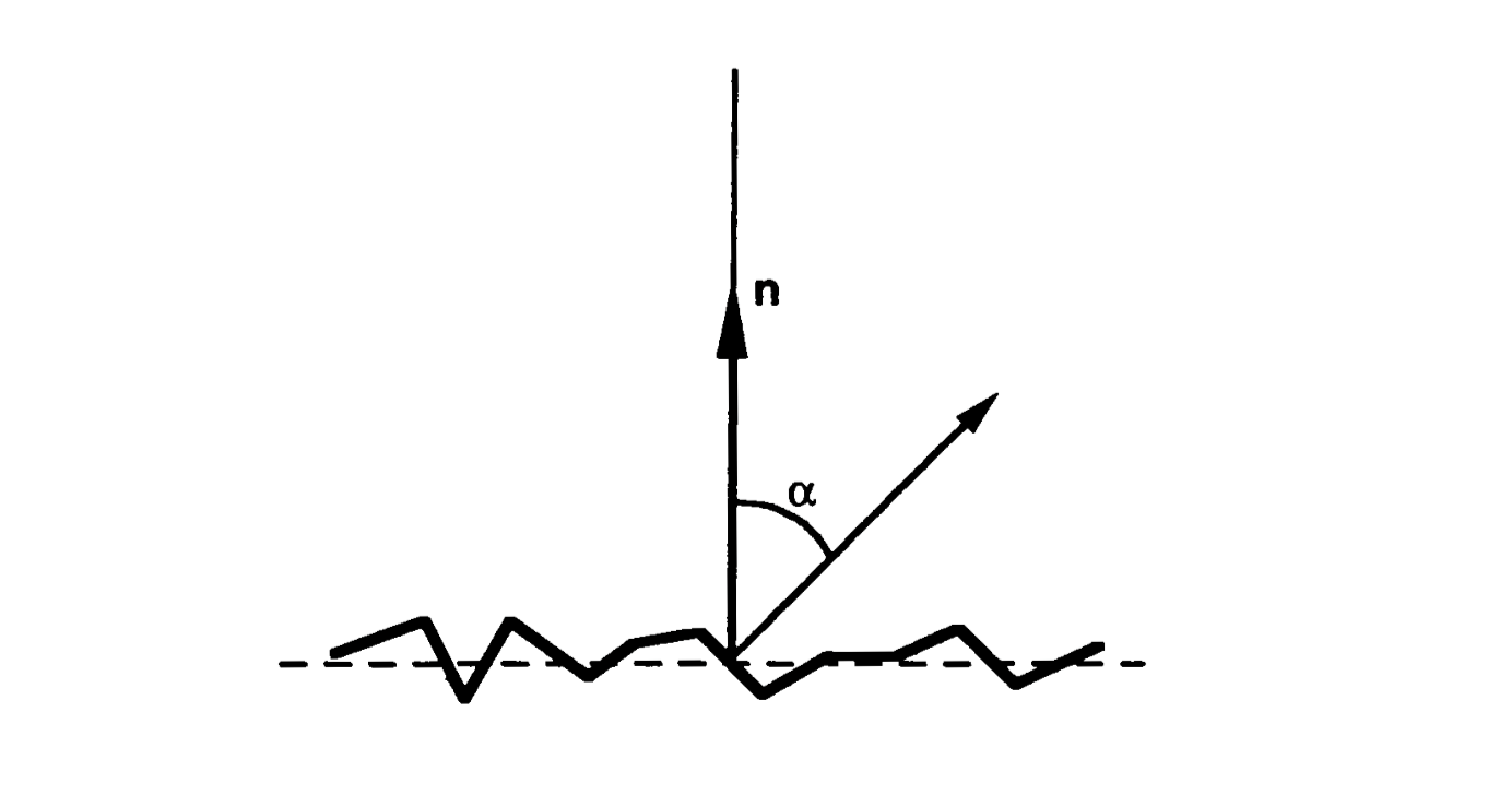
A large set of micro-facets constitutes an infinitesimal surface patch that has a mean surface orientation \(\vec{n}\). Each micro-facet has its own orientation, which may deviate from the mean surface orientation by an angle \(\alpha\).
We will use the parameter \(\alpha\) to represent the slope of individual facets. Surfaces can be modeled by a statistical distribution of the micro-facet slopes. If the surface is isotropic, the probability distribution of the micro-facet slopes can be assumed to be rotationally symmetric w.r.t the mean surface normal \(\vec{n}\). Therefore, facet slopes can be described by a one-dimensional probability distribution function. For instance, the surface may be modeled by assuming a normal distribution for the facet slope \(\alpha\), with mean value \(\bar{\alpha}=0\) and standard deviation \(\sigma_\alpha\):
\[p_\alpha(\alpha)=\frac{1}{\sqrt{2\pi}\sigma_\alpha}e^{-\frac{\alpha^2}{2\sigma_\alpha^2}}\]The surface model is determined by a single parameter \(\sigma_\alpha\), and larger \(\sigma_\alpha\) can be used to model rougher surfaces. While autocorrelation coefficient is important, the concept of slope correlation is more difficult to interpret and is not that useful in the generation of surface, which results in a weaker model compared to the height model. However, slope distribution model is popular in the analysis of surface reflection, as the scattering of light rays is dependent on the local slope of the surface and not the local height of the surface.
Surface roughness
Surface reflection theory relates irregularities to the wavelength of incident light and the angle of incidence. For incident light of a given wavelength, the roughness of a surface may be estimated by studying the manner in which the surface scatters light in different directions. If the surface irregularities are small compared to the wavelength of incident light, a large fraction of the incident light will be reflected specularly in a single direction. If the surface irregularities are large compared to the wavelength, the surface will scatter the incident light in various directions. Conversely, the same surface can be made to appear smooth or rough by varying the wavelength of incident light; or for the same wavelength it can be made to appear smooth or rough by varying the angle of incidence.
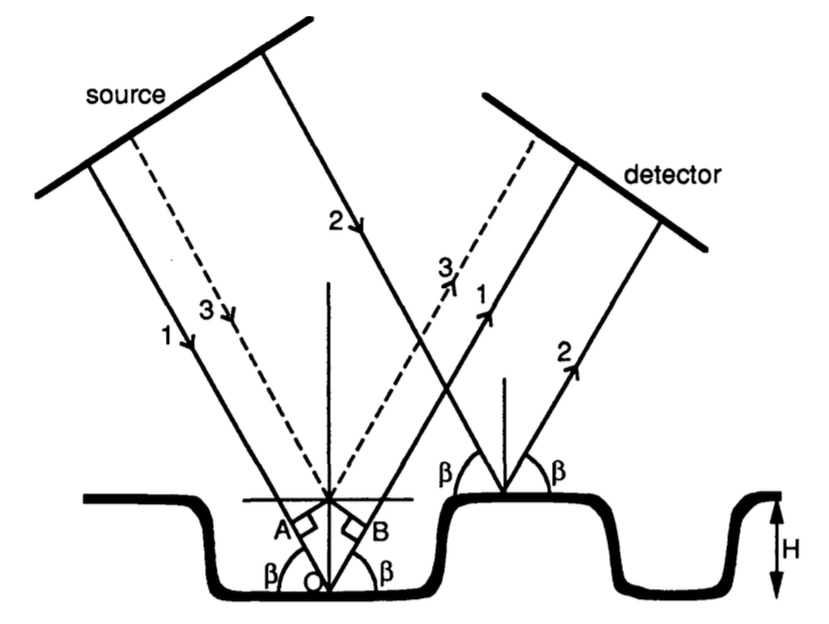
Raleigh suggested a way of relating surface roughness to wavelength and angle of incidence, and established a simple criterion for classifying surfaces as smooth or rough. Consider ray 1 and ray 2 in the figure above, incident at an angle \(\beta\) on a surface with irregularities of height \(H\). Since the two rays strike the surface at locally smooth patches, both rays are specularly reflected. The rays originate from a source plane that is perpendicular to the rays, and they are received by a detector that is perpendicular to the reflected rays. We are interested in finding the difference between the paths traveled by the two rays. We can get
\[\begin{align} \Delta d&=AOB\\ &=2Hsin\beta \end{align}\]If \(\lambda\) is the wavelength of the incident rays, the phase difference between the rays received by the detector may be determined from the path difference as:
\[\Delta \Omega = \frac{4\pi H}{\lambda}sin\beta\]If \(\Omega\) is small, the two rays received by the detector will be almost in phase with each other, and the received energy will be nearly equal to the sum of the energies carried by the two rays. In this case, the surface reflects light specularly and is thus smooth.
If \(\Omega\) approaches \(\pi\), the two rays will be in phas opposition and will tend to cancel the effects of each other. If \(\Omega=\pi\), no energy will flow in the direction of the detector. The incident energy is thus redistributed in other directions, and thus rough.
By selecting a threshold value of \(\frac{\pi}{2}\), we have Raleigh criterion that states that a surface is considered to be rough when:
\[H>\frac{\lambda}{8sin\beta}\]BRDF
BRDF is short for Bidirectional Reflectance Distribution Function. It’s defined as
The ratio of the radiance in the outgoing direction to the incident irradiance.
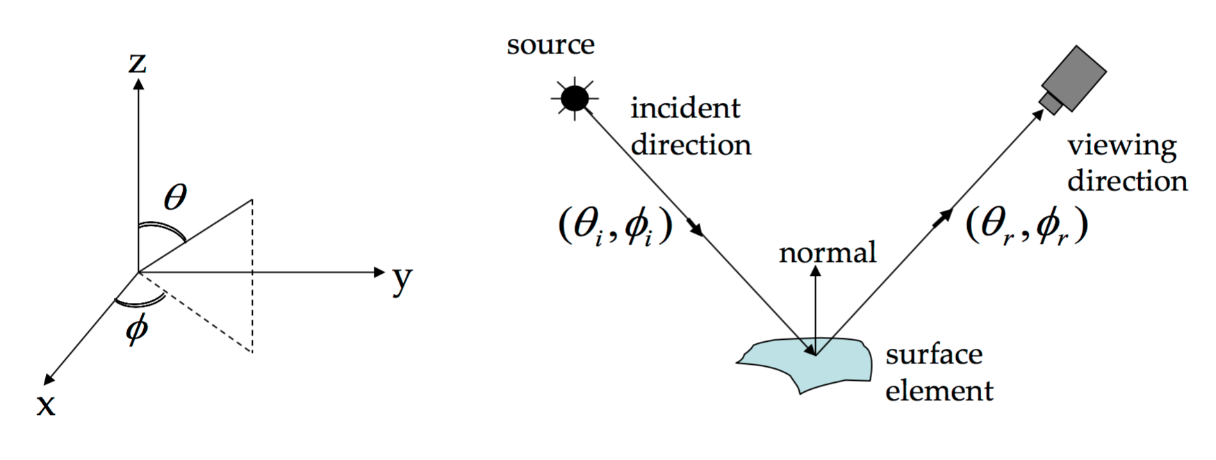
\[f(\theta_i, \phi_i; \theta_r, \phi_r) = \frac{L^{surface}(\theta_r ,\phi_r)}{E^{surface}(\theta_i, \phi_i)}\]
where \(L^{surface}(\theta_r ,\phi_r)\) is the radiance of surface in direction \(\theta_r ,\phi_r\), and \(E^{surface}(\theta_i, \phi_i)\) is irradiance at surface in direction \(\theta_i, \phi_i\)
Properties
The term physically plausible BRDF is used for reflectance functions that satisfy energy conservation and reciprocity.
- Energy Conservation: the integral of BRDF over all outgoing directions, scaled by the cosine term to accout for foreshortening, must be less than 1.
- Helmholtz Reciprocity: BRDF doesn’t change when source and viewing directions are swapped, which is due to the symmetry of light transport.
Some, but not all, BRDFs have a property called isotropy: they are unchanged if the incoming and outgoing directions are rotated by the same amount about the surface normal. In this case, the BRDF is a 3D function, and depends only on the difference between the azimuthal angles of incidence and exitance.
Constraints
The total energy arriving at a surface patch \(dA\) in a time interval \(dt\) is
\[(\int_{\Omega_i} L_i(P, \theta_i, \phi_i)cos\theta_i d\omega_i)dA dt = \int_0^{2\pi} \int_0^{\pi/2} L_i(P, \theta_i, \phi_i)cos\theta_i sin\theta_i d\theta_i d\phi_i)dA dt\]We assume that any energy leaving at the surface leaves from the same point at which it arrived and no energy is generated within the surface. This means that the total energy leaving the surface during that interval is less than or equal to the amount arriving. This means, the inequality must hold, whatever the choice of \(L_i\).
\[\begin{align} (\int_{\Omega_i} L_i(P, \theta_i, \phi_i)cos\theta_i d\omega_i)dA dt & \geq (\int_{\Omega_r} L_o(P, \theta_r, \phi_r)cos\theta_r d\omega_r)dA dt\\ & \geq (\int_{\Omega_r} \int_{\Omega_i} f(\theta_i, \phi_i; \theta_r, \phi_r) L_i(P, \theta_i, \phi_i)cos\theta_i d\omega_i cos\theta_r d\omega_r)dA dt \end{align}\]Representation [1]
The main efforts in BRDF representation have focused on either analytic formulas that can represent some narrow class of BRDFs, or generic techniques suitable for storing arbitrary 4D functions.
Analytic model - Physically-based and Phenomenological
Many of these analytic models are the result of modeling the properties of a real surface and mathematically computing the amount of light that would be reflected by a surface with those properties. For example, physically-based BRDFs have been derived for primarily specular surfaces (e.g. the Cook-Torrance-Sparrow model), for rough diffuse surfaces (the Oren-Nayar model), and for dusty surfaces (the Hapke/Lommel-Seeliger model). Those physically-based models, to a large degree, satisfy the criteria of physical plausibility.
An inherent property of physically-based models is that because they start with specific assumptions about microgeometry, they can only predict the reflectance of surfaces that closely match those assumptions. As a result, even the most elaborate theoretical models cannot predict reflectance from surfaces with complex microstructure or mesostructure.
Phenomenological models have been used to widen the range of representable BRDFs. For instance, Minnaert BRDF is used to model lunar reflection, Lafortune’s generalized cosine lobes can represent a wide range of phenomena.
Decomposition into Basis Functions
Describing a complex function as a linear combination of some set of basis functions is a widely used technique for representing continuous functions. The most classes of basis functions are tensor products of the spherical harmonics, Zernike polynomials, and spherical wavelets.
Spherical harmonics, the spherical analogue of sines and cosines, are a popular choice for representing BRDFs.
An alternative is to use a basis of functions on a disk, then map those functions onto a hemisphere. For instance, Zernike polynomials.
Both the spherical harmonics and Zernike polynomials require large numbers of basis functions in order to represent quickly-varying BRDFs accurately, and evaluating a BRDF represented in terms of these functions requires computation time proportional to the total number of nonzero coefficients.
Wavelets have been proposed as an alternative set of basis functions for BRDF representation, because they help reduce evaluation time and storage cost.
Change of Variables
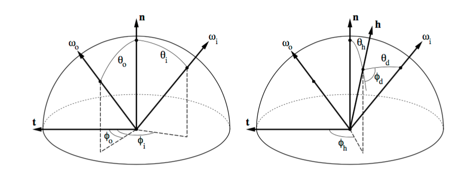
The transformation is a change of variables that causes some features of common BRDFs to lie along the new coordinates axes. Specifically, BRDF is parametrized in terms of the halfway vector (the vector halfway between the incoming and reflected rays) and a “difference” vector, which is just the incident ray in a frame of reference in which the halfway vector is at the north pole. That is, instead of representing the BRDF as \(f(\theta_i, \phi_i, \theta_r, \phi_r)\), we regard the BRDF as a function of the halfangle and difference angle: \(f(\theta_h, \phi_h, \theta_d, \phi_d)\), where
\[\begin{align*} \vec{n} &= \text{Surface normal,}\\ \vec{t} &= \text{Surface tangent (i.e. orientation of an anisotropic surface),}\\ \vec{b} &= \text{Surface binormal (i.e. }n \times t\text{),}\\ \vec{\omega}_i &= sph(\theta_i, \phi_i), \text{where } \theta_i \text{ is measure relative to } \vec{n} \text{ and } \phi_i \text{ is relative to } \vec{t}\\ \vec{\omega}_o &= sph(\theta_o, \phi_o)\\ \vec{h} &= sph(\theta_h, \phi_h)\\ &= \frac{\vec{\omega}_i + \vec{\omega}_o}{\|\vec{\omega}_i + \vec{\omega}_o\|}\\ \vec{d}&=sph(\theta_d, \phi_d)\\ &= rot_{\vec{b},-\theta_h}rot_{\vec{n},-\phi_h}\vec{\omega}_i \end{align*}\]Note that \((\theta_h, \phi_h)\) are the sphercial coordinates of the halfway vector in the \(\vec{t}-\vec{n}-\vec{b}\) frame. The two rotations brings the halfangle \(\vec{h}\) to the north pole, and \(\theta_d, \phi_d\) are the spherical coordinates of the incident ray in this transformed frame.
Properties in the New Coordinates
- Isotropic BRDF is a constant function of \(\phi_h\), and independent of \(\phi_h\), which means that an isotropic BRDF will have basis function coefficients equal to zero for all basis functions that vary with \(\phi_h\).
- The angles of incidence and reflection become much more symmetric. In particular, the condition of Helmholtz reciprocity becomes a simple symmetry under \(\phi_d \Rightarrow \phi_d + \pi\).
- Ideal specular and near-ideal specular peaks are transformed by the change of variables to lie mostly along the \(\theta_h\) axis. An ideal specular peak is represented as a delta function of \(\theta_h\), and is completely independent of the other three variables. In general, any BRDF that depends only on \((\vec{n} \cdot \vec{h})\) is independent of three of the four variables in the transformed sapce.
- Any analytic model that starts with an isotropic microfacet distribution and ignores masking, shadowing, and interreflectance will be a separable function of only \(\theta_h\) and \(\theta_d\) in the transformed coordinates.
- Retroreflective peaks are transformed to be functions of only \(\theta_d\).
Special Cases
Radiosity
If the radiance leaving a surface is independent of exit angle, there is no point describing it as a unit that explicitly depends on direction. The appropriate unit is radiosity (\(B(P)\)), defined as
the total power leaving a point on a surface per unit area on the surface
To compute the radiosity of a surface point, we can sum the exit radiance over the whole hemisphere.
\[B(P) = \int_\Omega L(P, \theta, \phi) cos\theta d\omega\]Directional Hemisphere Reflectance
The light leaving many surfaces is largely independent of the exit angle. A natural measure of a surface’s reflective properties is the directional-hemispheric reflectance, defined as
the fraction of the incident irradiance in a given direction that is reflected by the surface, whatever the direction of the reflection.
The directional hemispheric reflectance is obtained by summing the radiance leaving the surface over all directions and dividing by the irradiance in the direction of illumination, thus it’s dimensionless, and ranges from 0 to 1.
\[\begin{align} \rho(\theta_i, \phi_i) &= \frac{\int_\Omega L_r(P, \theta_r, \phi_r)cos\theta_r d\omega_r}{L_i(P, \theta_i, \phi_i)cos\theta_i d\omega_i}\\ &=\int_\Omega \{\frac{L_r(P, \theta_r, \phi_r)cos\theta_r}{L_i(P, \theta_i, \phi_i)cos\theta_i d\omega_i}\}d\omega_r\\ &=\int_\Omega f(\theta_i, \phi_i, \theta_r, \phi_r)cos\theta_r d\omega_r \end{align}\]Scene Radiance Equation (very important)
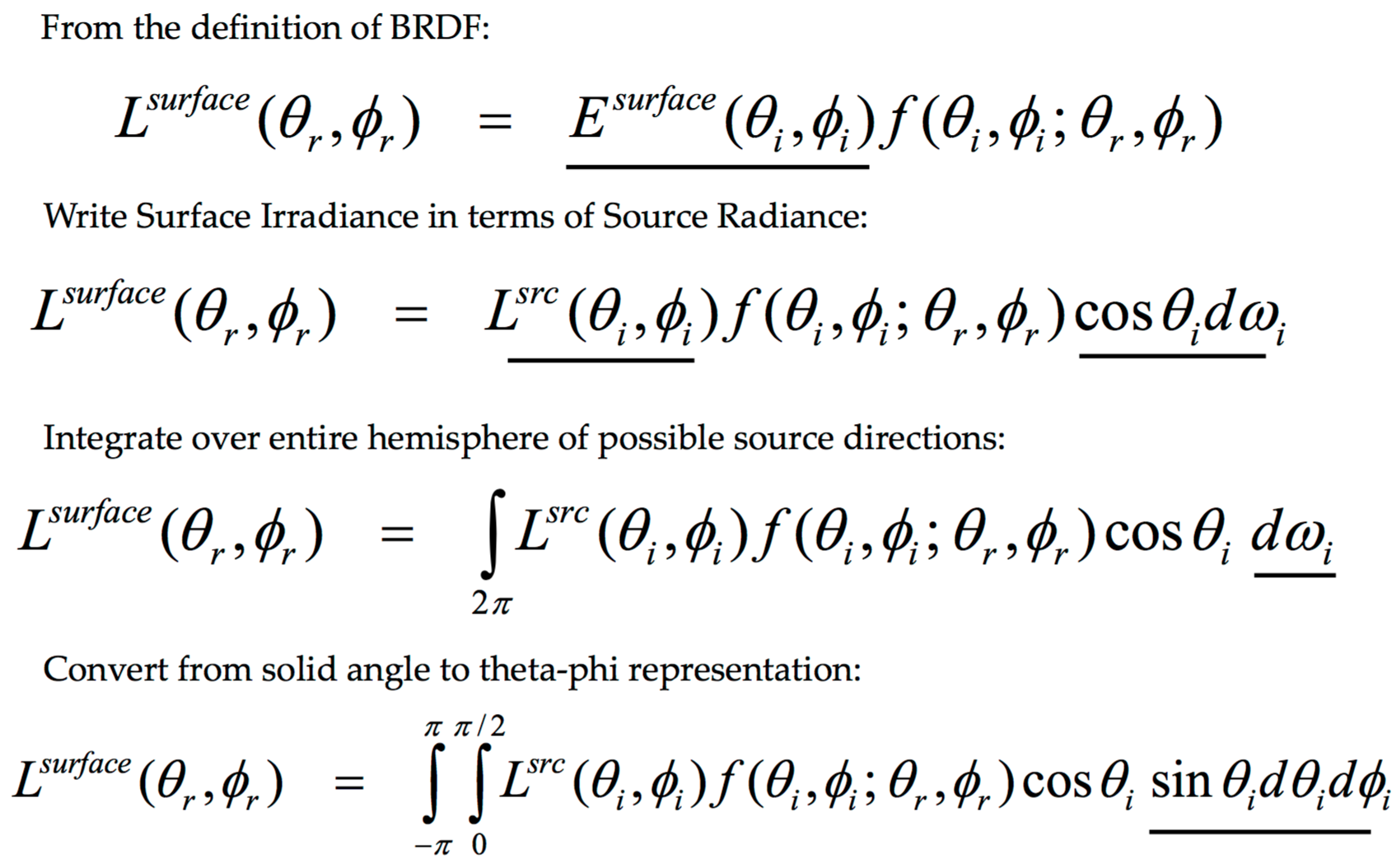
Reflection Model
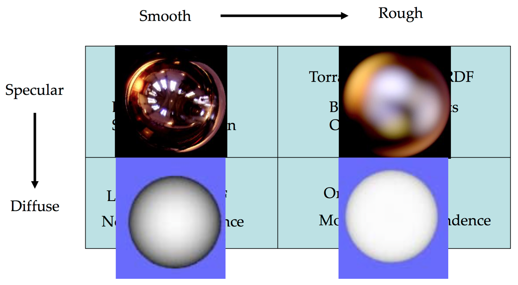
Diffuse reflection from Smooth Surfaces
- Lambertian BRDF is a constant, independent of incoming or outgoing direction: \(f(\theta_i, \phi_i; \theta_r, \phi_r)=\frac{\rho_d}{\pi}\), where \(\rho_d\) is the diffuse albedo (a special case of directional hemispherical reflectance)
- Surface Radiance: \(L=\frac{\rho_d}{\pi}Icos\theta_i=\frac{\rho_d}{\pi}I\vec{n} \cdot \vec{s}\), where \(I\) is source intensity.

Radiance decreases with increase in angle between surface normal and source direction. Thus the edge of a Lambertian object should be dark (\(\vec{n} \cdot \vec{s}=0\)).
Conflict: The moon appears diffuse, but the edges of the moon look bright when illuminated by earth’s radiance.
Fact: Surface roughness causes flat appearance, e.g. the full moon has a flat appearance. The roughness increase from left to right in the following image
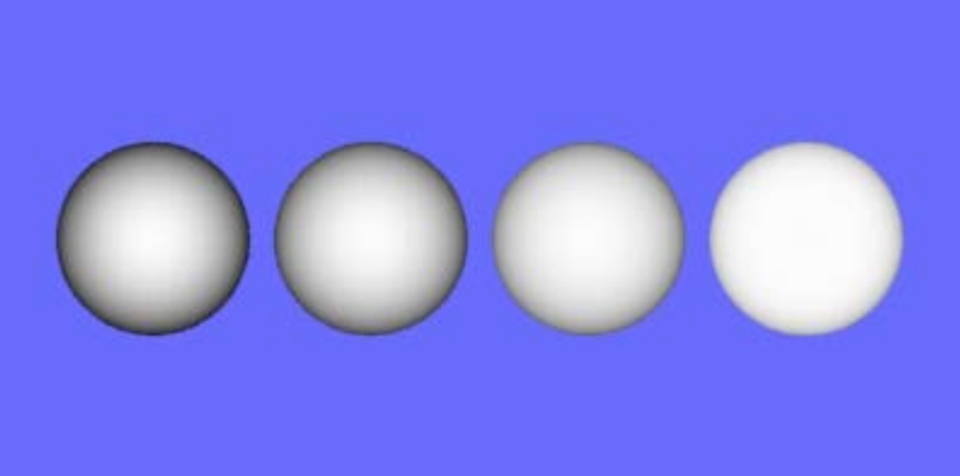
Lambertian model is valid for only smooth matte surfaces, bad for rough matte surfaces (like the moon).
Diffuse Reflection from Rough Surfaces
Oren-Nayar Model
[TBD]
Specular reflection from Smooth Surfaces
- Very smooth surface, all incident light is reflected in a SINGLE direction.
- Mirror BRDF is a double-delta function: \(f(\theta_i, \phi_i; \theta_r, \phi_r)=\rho_s\delta(\theta_i-\theta_v)\delta(\phi_i+\pi-\phi_v)\), where \(\rho_s\) is the specular albedo.
- Surface Radiance: \(L = I\rho_s\delta(\theta_i-\theta_v)\delta(\phi_i+\pi-\phi_v)\)
Specular Reflections from Rough Surfaces
Specular lobes (specularity)
Radiation arriving in one direction leaves in a small lobe of directions around the specular direction, which results in a blurring effect. The most common model used to model the shape of the lobe is the Phone model.
Phone Model
In this model, the radiance leaving a specular surface is proportional to \(cos^n(\sigma\theta)=cos^n(\theta_r-\theta_s)\), where \(\theta_r\) is the exit angle, and \(\theta_s\) is the specular direction and \(n\) is a parameter. large values of \(n\) lead to a narrow lobe and small, sharp specularities; small values lead to a broad lobe and large specularities with rather fuzzy boundaries.
- Sort of works, easy to compute
- Not physically based (no energy conservation and reciprocity)
- Commonly used in CG
Torrance-Sparrow Model
- Physically based model for surface reflection
- Based on geometric optics
- Explains off-specular lobe (wider highlights)
- Works for only rough surfaces
[TBD]
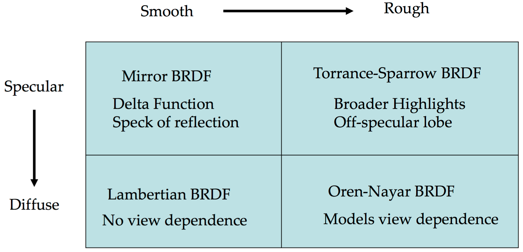
Summary of Surface and BRDFs
Reference
[1] Rusinkiewicz. A New Change of Variables for Efficient BRDF Representation
[2] Nayar, Ikeuchi, Kanade. Surface Reflection: Physical and Geometrical Perspectives