Content-based Video Copy Detection - a step by step walkthrough
This tutorial is based on the code released for ViSiL: Fine-grained Spatio-Temporal Video Similarity Learning. Please refer to the paper for more technical details.
Introduction
Visil computes the video to video similarity score in three steps: 1) feature extraction, 2) frame-to-frame similarity, 3) video-to-video similarity. See the image below for an overview of the workflow.

Feature extraction
Extract features from the intermediate convolution layers of a CNN architecture by applying region pooling on the feature maps (turns CNN feature map to a fixed size map). An PCA and attention layer could be applied to whiten and re-weight the features.
Given a video of $P$, the input is $P\times H\times W\times C$, where $H$, $W$ is the height and width of the video frame. The output of the CNN is $P\times N\times N\times C$, where $N$ is the output size of the region pooling layer, and $C$ is the total number of intermediate convolution layers.
When we use ResNet-50 as our backbone, the feature map extracted from one video is $P\times 3\times 3\times 3840$, or it can also be rearranged to be $P\times 9\times 3840$.

Frame-to-Frame similarity
Given two frame $d$, $b$ and their corresponding feature map $M_d, M_b \in \mathbb{R}^{NxNxC}$. The region map can be decomposed into region vectors $d_{ij}, b_{kl} \in \mathbb{R}^C, i,j,k,l \in [1,N]$. Then the dot product between every pair of region vectors is calculated, creating a similarity matrix of the two frames. Chamfer similarity (CS) is applied on the similarity matrix to compute the frame-to-frame similarity
\[CS(d, b) = \frac{1}{N^2} \sum_{i,j=1}^N \max_{k,l\in[1,N]} d_{ij}^\top b_{kl}\]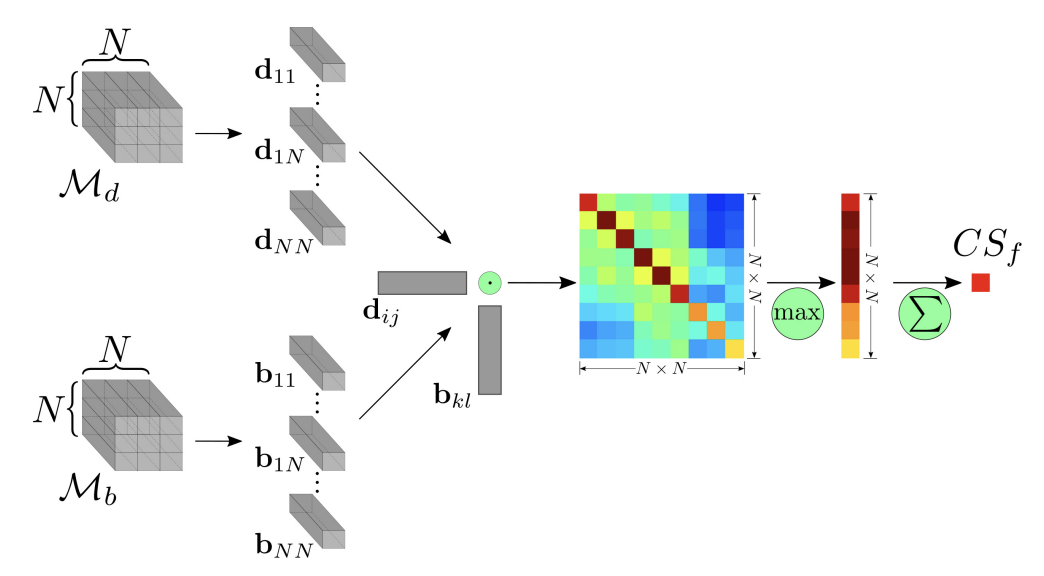
Video-to-Video similarity
Given two videos $X, Y$ with $P, Q$ frames respectively, we compute pairwise frame-to-frame similarity for all frames between these two videos and derive the frame-to-frame similarity matrix $S(X, Y)\in ℝ^{P \times Q}$
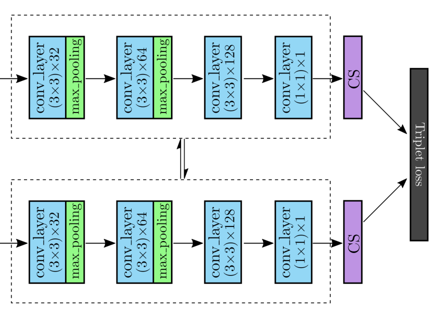
Then we feed the frame-to-frame similarity matrix to a CNN to train a video level similarity model using triplet loss. We use a harh tanh to clip the output the network within $[-1, 1]$ and use triplet score as our loss function.
Walkthrough
Load model
Install the [visil] package following this guide.
from model.visil import ViSiL
from utils import load_video

model = ViSiL(pretrained=True)
model = model.to(device)
model.eval()
Prepare dataset
In this notebook, we use the FIVR-200K dataset, which comprises 225,960 videos associated with 4,687 Wikipedia events and 100 selected video queries.
This dataset has been collected for the problem of Fine-grained Incident Video Retrieval (FIVR), of which the objective is to retrieve all associated videos given a query video. There are three association types considered:
- Duplicate Scene Videos (DSV): Videos that share at least one scene (captured by the same camera) regardless of any applied transformation.
- Complementary Scene Videos (CSV): Videos that contain part of the same spatio-temporal segment, but captured from different viewpoints.
- Incident Scene Videos (ISV): Videos that capture the same incident, i.e. they are spatially and temporally close, but have no overlap.
To make this demo more tractable, we use a small set of videos (5 scenes, 5 videos for each scene, a total of 25 videos) as a demonstrative purpose. For each scene, there are:
- an anchor video
- a Near Duplicate video (ND)
- a Duplicate Scene video (DS)
- a Complementary Scene video (CS)
- a Incident Scene video (IS)
If our system works properly, it should find the ND, DS and CS video given the anchor video (the IS has no overlapping frames with the anchor video).
Download videos
Install the [FIVR-200K] package following this guide
# Install yt-dlp to download YouTube videos
!python3 -m pip install -U yt-dlp

video_id_path = '<your-video-id-path>'
video_path = '<your-video-path>'
if not os.path.exists(video_path):
  !mkdir -p $video_path
  !python download_dataset.py --video_dir $video_path --dataset_ids $video_id_path --cores 4 --resolution 360
Content-based video copy detection: a brute-force approach
In this section, we will go through the process of 1) generating frame feature map; 2) compute frame-to-frame similarity score between two frames and similarity matrix for two videos; 3) compute video-to-video similarity score.
This section should give you a sense of all the basic ingredients of a similar video detection system without diving deep into the technical details.
Extract Frame Feature Map
There are many ways of extracting features from videos, and they can be roughly divided into video-level features and frame-level features. Our approach falls into the second category, thus it consists of
- extract (key) frames from a video;
- extract frame feature map for a frame.
There are many different algorithms for these two steps. For this demo, we opt to extract one frame per second given a video and use a pre-trained CNN for feature extraction.
# Extract frame from video.
query_video = torch.from_numpy(load_video(video_name(video_ids[0])))
target_video = torch.from_numpy(load_video(video_name(video_ids[3])))
query_video.shape, target_video.shape
# Extract frame feature map from video frames.
query_features = model.extract_features(query_video.to(device))
target_features = model.extract_features(target_video.to(device))
query_features.shape, target_features.shape
As we can see from the above two examples, the query video has shape of $59 \times 9 \times 3840$ while the target video has shape of $78 \times 9 \times 3840$. Below is a brief intro of what these numbers mean w/o needing to understand the underlying model.
- 1st number: number of video frames
- 2nd number: output of Region Pooling layer. ($H \times W → 3\times 3$)
- 3rd number: number of filters/kernels from all conv layers
# Extract features for all videos and save them in file.
# NOTE: only need to run once since the features are saved on file.
feature_path = '%s/visil/features' % GIT_REPO_PATH
if not os.path.exists(feature_path):
  !mkdir -p $feature_path

for video_id in video_ids:
  feature_file = '%s/%s.pt' % (feature_path, video_id)
  if os.path.exists(feature_file):
    continue
  video = torch.from_numpy(load_video(video_name(video_id)))
  if device.type == 'cuda':
    features = model.extract_features(video.to('cuda'))
  else:
    features = model.extract_features(video)

  torch.save(features, feature_file)
# Load all features in a map (video id => features).
feature_path = '%s/visil/features' % GIT_REPO_PATH
vid2feature = {}
for video_id in video_ids:
  feature_file = '%s/%s.pt' % (feature_path, video_id)
  vid2feature[video_id] = torch.load(feature_file, map_location=device)
len(vid2feature)
Compute Frame-to-Frame Similarity Matrix
As mentioned above, given a frame level feature from the query and target video respectively, the frame-to-frame similarity score between these two frames can be computed using the following pseduocode:
def f2f_simi_score(frame_1, frame_2):
  for region_vec_1 in frame_1:
    for region_vec_2 in frame_2:
      max_simi = max(max_simi, simi_score(region_vec_1, region_vec_2))
    sum_simi += max_simi

  return sum_simi / len(frame_1)
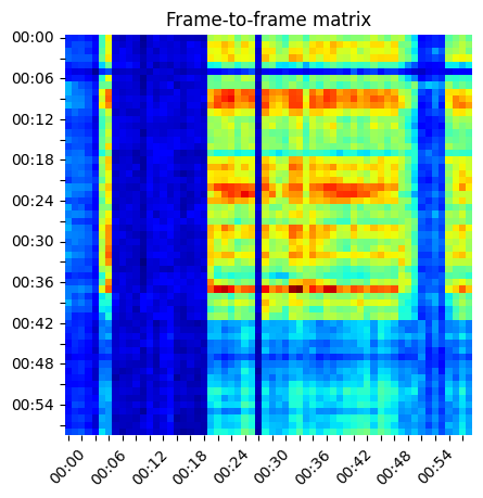
Since there are $Q$ frames in the query video and $T$ frames from the target video, there are $Q \times T$ pairs of frames, and thus a frame2frame similarity matrix of size $(Q, T)$.
Caveat: as we can see from the pseduocode, f2f_simi_score is not commutative, i.e., f2f_simi_score(frame_1, frame_2) != f2f_simi_score(frame_2, frame_1). We won’t discuss apporaches to address this issue since it’s out of the scope of this demo.
def visualize_matrix(sim_matrix, title, step=1):
  # create a heatmap based on the input similarity matrix
  ax = sns.heatmap(sim_matrix, cmap="jet", cbar=False, square=True)

  # set axes ticks
  ax.set_xticklabels(map(lambda s: "%02d:%02d" % divmod(s*step, 60), ax.get_xticks()-0.5))
  for ind, label in enumerate(ax.get_xticklabels()):
      label.set_visible(ind % 3 == 0)
  ax.set_yticklabels(map(lambda s: "%02d:%02d" % divmod(s*step, 60), ax.get_yticks()-0.5))
  for ind, label in enumerate(ax.get_yticklabels()):
      label.set_visible(ind % 2 == 0)

  plt.xticks(rotation=45)
  plt.yticks(rotation=0)
  plt.title(title)

  plt.show()

sim_matrix = model.calculate_f2f_matrix(query_features[None, :], target_features[None, :])
if device.type == 'cuda':
  sim_matrix = sim_matrix.detach().to('cpu')
visualize_matrix(sim_matrix[0], 'Frame-to-frame matrix')
Compute Video-to-Video Similarity
The frame2frame similarity matrix is passed to another CNN to learn the spatial temporal relationship between these similarity scores, and the video2video score is computed as follows:
def v2v_simi_score(f2f_simi_score):
  m, n = f2f_simi_score.shape

  for i in [0...m):
    for j in [0...n):
      max_simi = max(max_simi, f2f_simi_score[i][j])
    sum_simi += max_simi

  return sum_simi / m
sim_matrix = model.calculate_visil_output(query_features[None, :], target_features[None, :])
if device.type == 'cuda':
  sim_matrix = sim_matrix.detach().to('cpu')
visualize_matrix(sim_matrix[0], 'ViSiL output', step=4)
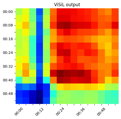
Interpretation video-to-video similarity: given a query video 𝑄 and a target video 𝑇 , the v2v similarity can be interpreted as the ratio of query video 𝑄 that can be matched in the target video 𝑇 .
Compute pairwise Video-to-Video similarity
import numpy as np

num_videos = len(video_ids)
similarity_matrix = np.zeros((num_videos, num_videos))

for i in range(num_videos):
  video_id_i = video_ids[i]
  for j in range(i, num_videos):
    video_id_j = video_ids[j]
    similarity_matrix[i][j] = model.calculate_video_similarity(vid2feature[video_id_i].to(device), vid2feature[video_id_j].to(device))
import pandas as pd

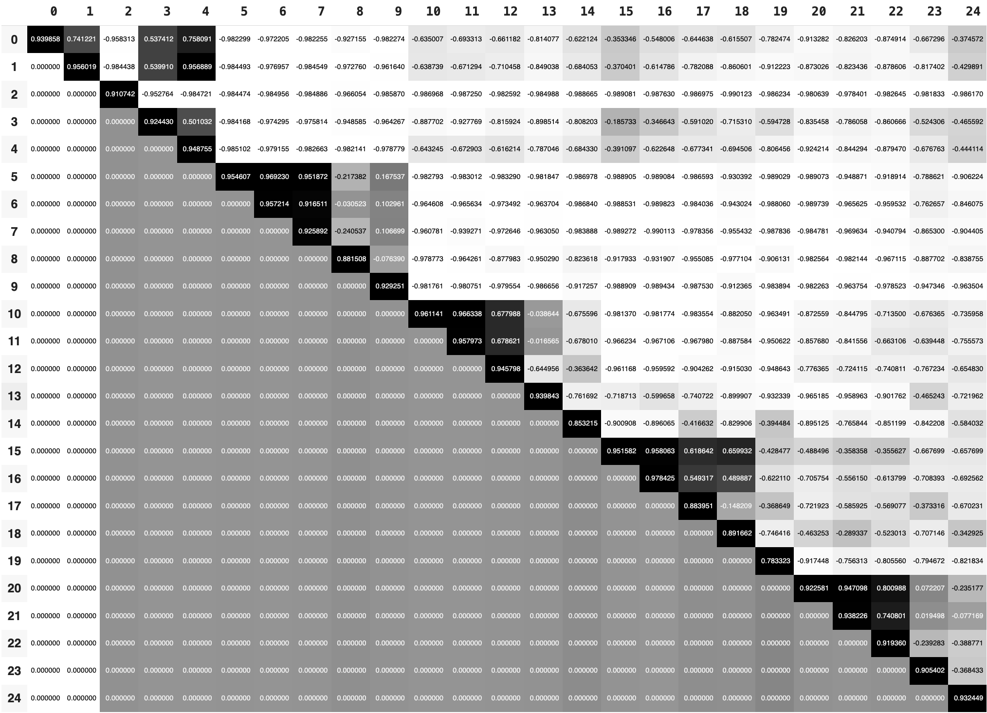
df = pd.DataFrame(similarity_matrix)
df.style.set_properties(**{'font-size':'6pt'}).background_gradient('Greys')
Similar Video Detection: An Hierarchical Approach
In the previous section, we built a small yet fully functional similar video detection system, but the approach has a time and space complexity of $O(QT)$ for just two videos, which is not practical in real-world application.
We draw inspiration from a typical modern recommendation system, which typically has three components: 1) a feature extraction pipeline, 2) a candidate generation pipeline that generates tens of thousands of candidates from potentially millions of samples, 3) a scoring system that ranks the candidates.
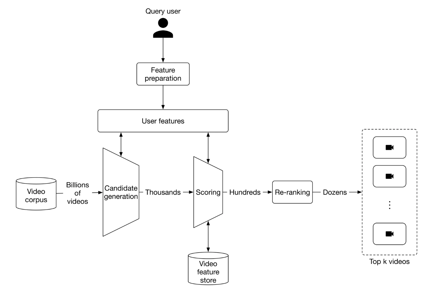
In this section, we will discuss how to find the most likely candidates using nearest neighbor search. An alternative two-step approach is proposed as follows:
- Extract features for each frame given a video, and store it in file;
- Find a list of candidate videos to narrow down the search range;
- Find all matched videos given a query video, ranked by similarity score.
Generate candidates
Aggregate frame features from all videos.
num_videos = len(video_ids)
all_features = []
all_frames = [] # frame info: (video id, frame idx)
feat2vid = {} # frame feature SHA => video id

for i in range(num_videos):
  video_id = video_ids[i]
  features = vid2feature[video_id].view(-1, 9*3840)

  all_features.append(features)
  all_frames.extend([(video_id, frame_idx) for frame_idx in range(features.shape[0])])

  f2v = {hash_tensor_1d(idx, f) : video_ids[i] for idx, f in enumerate(features)}
  assert len(f2v) == features.shape[0], f"{video_ids[i]}: {len(f2v)}, {features.shape[0]}"
  feat2vid.update(f2v)

all_features = torch.cat(all_features, 0)
print('num of frames: %d, num of frame features %d' % (len(all_frames), all_features.shape[0]))
Here is an efficient method that computes the distance matrix between two frame feature map, which is used later to compute distance between two features.
def calc_pairwise_dist(features1, features2):
  N, D = features1.shape
  T, _ = features2.shape
  assert features1.dtype == features2.dtype
  dtype = features1.dtype
  return torch.matmul(features1**2, torch.ones((D, T), dtype=dtype)) + torch.matmul(torch.ones((N, D), dtype=dtype), torch.t(features2**2)) - 2 * torch.matmul(features1, torch.t(features2))
Compute the frame-to-frame distance matrix between the query video and all videos in the dataset. Sort the distance in ascending order.
import pandas as pd

query_video_id = video_ids[10]
features = vid2feature[query_video_id]
features = features.view(-1, 9*3840)

dist_matrix = calc_pairwise_dist(features.cpu(), all_features.cpu())
sorted_dist_matrix, indices = torch.sort(dist_matrix, dim = 1, descending=False) # Ascending order

df = pd.DataFrame(sorted_dist_matrix[:10, 0:120].detach().numpy())
df.style.set_properties(**{'font-size':'6pt'}).background_gradient('Greys')
Filter frame features whose distance to the query video frame is over a pre-defined threshold
dist_thresh = 4.0
mask = sorted_dist_matrix < dist_thresh

indices_tmp = indices.detach().clone()
indices_tmp[~mask] = -1

df = pd.DataFrame(indices_tmp[:10, 0:120].detach().numpy())
df.style.set_properties(**{'font-size':'6pt'}).background_gradient('Greys')
Find the similar videos
# Find the indices of all the matching frame whose distance to a query video frame is below a threshold.
selected_indices = torch.masked_select(indices, mask)
len(selected_indices)

# Find all the candidate videos
matched_video_ids = [all_frames[i][0] for i in selected_indices]

# Dedup matched video ids
unq_matched_video_ids = []
for id in matched_video_ids:
  if id not in unq_matched_video_ids:
    unq_matched_video_ids.append(id)
unq_matched_video_ids, len(unq_matched_video_ids)
Dimension reduction
Curse of Dimensionality
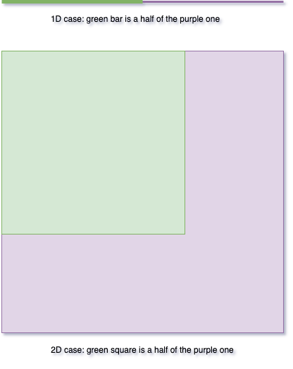
The curse of dimensionality is that as we increase the dimensionality of space, our data space becomes more and more sparse and so adding one more dimension would require an exponential increase in the number of sample data points to have the same sparsity. Please refer to the wiki page for more details.
Here is a simple illustration to demonstrate this effect: for the 1D case, we need to sample half of each dimension to retrieve half of all data samples; for the 2D case, we need to sample more than half of each dimension ($\frac{\sqrt{2}}{2}$ to be exact) to retrieve half of all data samples.
Please refer to A Dimension Reduction Technique to Preserve Nearest Neighbors on High Dimensional Data for a reference.