Documentation
Table of content
- Overview of real-world dataset
- Real-world MVS data
- Real-world PS data
- Real-world SL data
- Real-world VH data
- Overview of synthetic dataset
- Synthetic data
- Evaluation
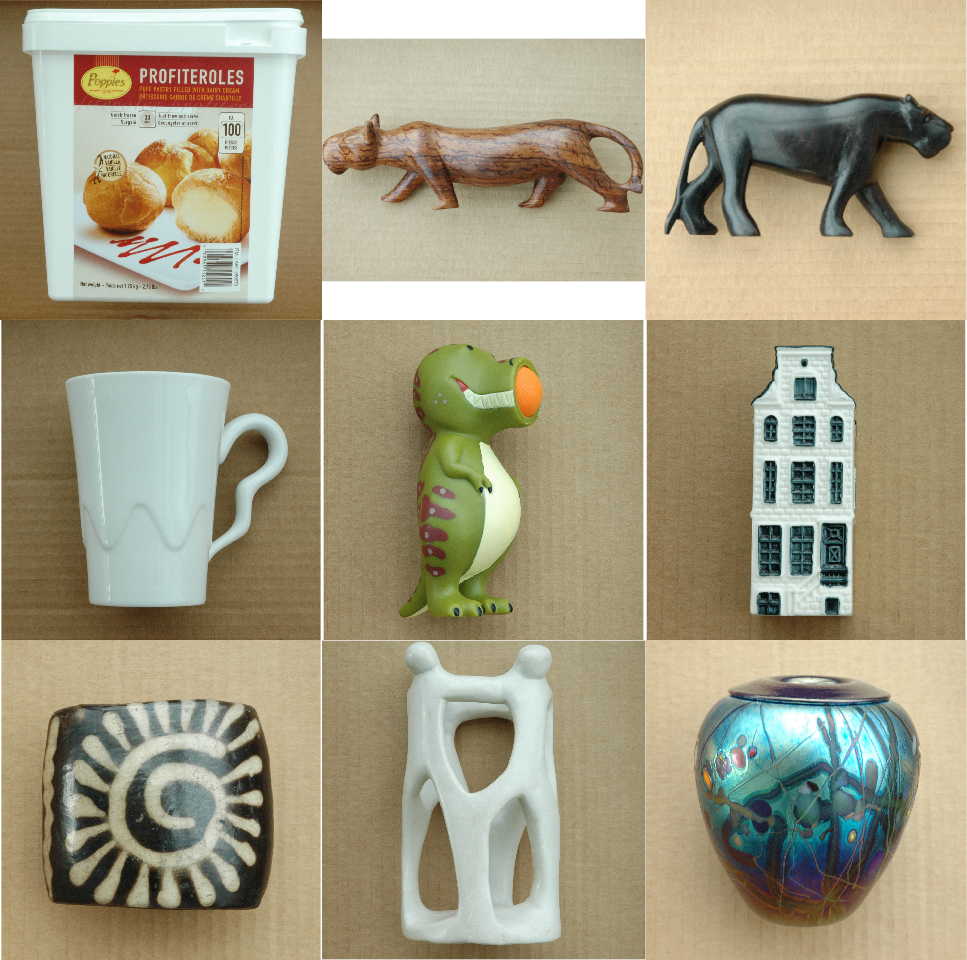
1. Overview of real-world objects
2. Real-world MVS data
The directory structure and naming convention are the same as those of PMVS. The directory structure is as follows:
.
├── model
├── txt
├── visualize
└── option.txt
2.1. Setup
For MVS, we capture the dataset by positioning the camera in three different heights. The objects are about 30-50cm away from the camera, and stays fixed on a turntable. We have followed the following two steps to acquire data: 1) put the camera at a different height, adjust the orientation so that the object in at the center of the frame; 2) take pictures while rotating the table. The table rotates approximately 30 every time. We rotate it 12 times and in total, we can obtain 12 image per height.
2.2. Calibratoin
For MVS, a calibration pattern proposed in Bo Li is imaged under the object, which is used for calibrating the camera position and orientation by Structure from Motion softwares, such as VisualSfM. The focal length is known a priori and remains fixed duing the image capturing process. Thus the extrinsic parameters of the camera can be retrieved up to a similarity transformation, and the reconstruction result is a metric/euclidean recontruction.
2.3. Data format
Images are captured by Nikon D70S camera with a lens in the jpeg format. The naming convension of images follows that of PMVS developed by Furukawa. For instance, the images are named as 00000000.xxx, 00000001.xxx, and so on. The images are stored in the visualize directory.
The txt directory contains the camera calibration results. The files must be named as 00000000.txt, 00000001.txt, and so on. The format of the camera parameter also follows that of PMVS, which is
CONTOUR
P[0][0] P[0][1] P[0][2] P[0][3]
P[1][0] P[1][1] P[1][2] P[1][3]
P[2][0] P[2][1] P[2][2] P[2][3]
3. Real-world PS data
The directory structure of PS dataset is as follows
.
├── ref_obj
|   └── 0000
|       ├── 000000xx.jpg
|       └── mask.bmp
|   └── 0001
|       ├── 000000xx.jpg
|       └── mask.bmp
├── 000000xx.jpg
├── mask.bmp
└── nomral.png
3.1. Setup
For PS, a 70-200mm lens, a handheld lamp, and two reference objects (dif- fuse and glossy) are used. The objects are positioned about 3m from the camera to approximate orthographic projection. To avoid inter-reflection, all data are cap- tured in a dark room with everying covered by black cloth except the target object. We use a hand-held lamp as the light source and choose close to frontal viewpoints to avoid severe self-shadowing effect. We take 20 images per object and select 15 plus images depending on the severity of the self-shadow effect.
3.2. Calibration
For most PS algorithms, i.e., calibrated PS algorithms, it is necessary to esti- mate the light direction and intensity. However, the selected PS algorithm can deal Appearance with unknown light sources and spatially-varying BRDFs. Thus, light calibration is not a required step. Though it is preferable to correct the non-linear response of camera, Hertzmann and Seitz discovered that it was unnecessary for EPS. Thus, we did not perform the radiometric calibration step. No geometric calibration of the camera is needed.
3.3. Data format
Images are captured by Nikon D70S camera with a lens in the jpeg format. Images are named following the convention: the first image is named as 00000000.xxx, the second is named as 00000001.xxx, and so on.
4. Real-world SL data
4.1. Setup
For SL, we use a Sanyo Pro xtraX Multiverse projector with a resolution of . The baseline angle of the camera projector pair is approximately 10 . To alleviate the effect of ambient light, all images are captured with room lights off. To counteract the effect of inter-reflection, additional images are captured by projecting an all-white and all-black patterns.
The Structure Light datasets contain images captured under the projection of column and row patterns. For each projection pattern, the reverse pattern is projected as well to eliminate the effects of global light transport. The resolution of the projector is 1024*768, thus, 10 temporally encoded patterns are needed. Two images with light on and off are captured to help the decoding process. Thus, the total number of images are .
4.2. Calibration
For SL, a opensource camera-projector calibration software developed by Moreno and Taubin is used for calibration. This technique works by projecting temporal patterns onto the calibration pattern, and uses local homography to individually translate each checkerboard corner from the camera plane to the projector plane. This technique can estimate both the intrinsic parameter and camera and projector, and the relative position and orientation.
4.3. Data formats
Images are captured by Nikon D70S camera with a lens in the jpeg or bmp format. Images are named following the convention: the first image is named as 0000.xxx, the second is named as 0001.xxx, and so on.
5. Overview of synthetic dataset
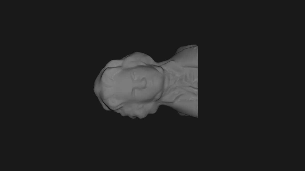
Bust
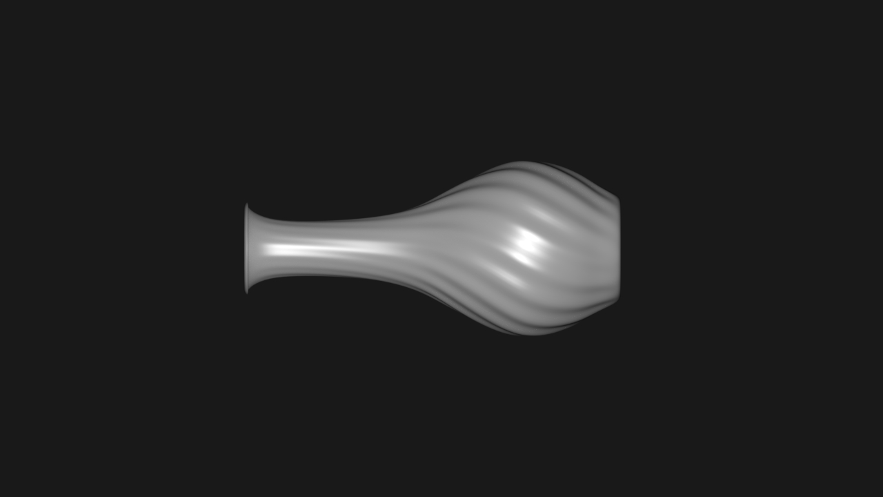
Vase 0
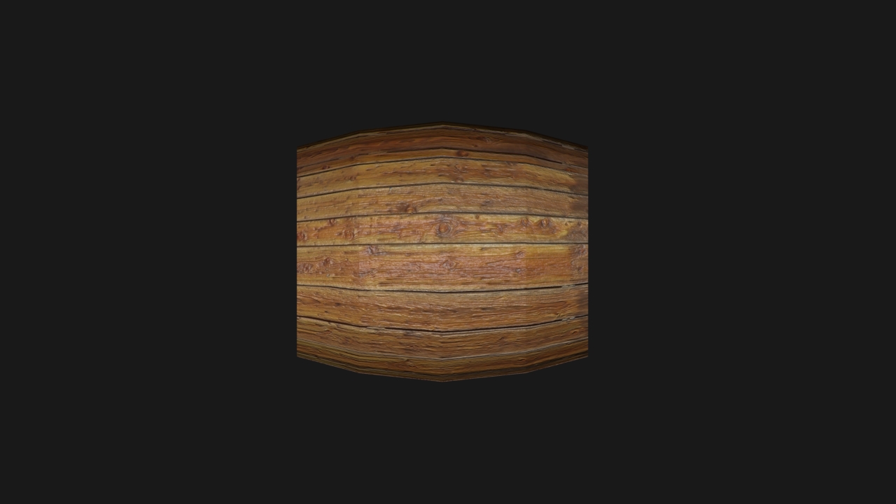
Barrel
Vase 1
6. Synthetic dataset
Synthetic data is used:
- discover the properties that have a significant main effect or interaction effect on algorithm performance (termed effective properties);
- evaluate algorithm performance under conditions consisting solely of effective properties;
- evaluate the performance of interprete.
6.1. Structure of dataset
Thus the structure of the first two synthetic datasets are similar, they have the following structure. The source code used to generate these dataset can be found in the Software page.
.
├── prob_cond_1
|    ├── mvs
|    ├── ps
|    └── sl
...
├── prob_cond_N
|    ├── mvs
|    ├── ps
|    └── sl
6.2. Effect of property
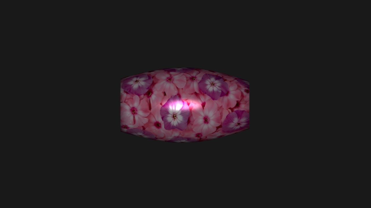
Here we show the visual effect of change each property from 0 to 1.


7. Evaluation
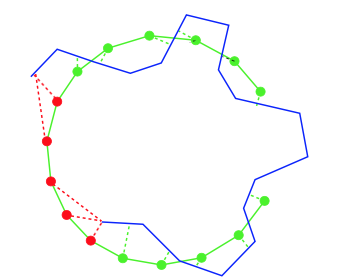
Accuracy: the distance between the points in the reconstruction and the nearest points on ground truth is computed, and the distance such that of the points on are within distance of is considered as accuracy. A reasonable value is between , and is set as . The lower the accuracy value, the better the reconstruction result. Note that as the accuracy improves, the accuracy value goes down.
Completeness: we compute the distance from to . Intuitively, points on are not covered if no suitable nearest points on are found. A more practical approach computes the fraction of points of that are within an allowable distance of . Note that as the completeness improves, the completeness value goes up.
Angular error: depth information is lost since only one viewpoint is used. Thus, the previous metrics are not applicable. Here we employ another evaluation criteria that is widely adopted, which is based on the statistics of angular error. For each pixel, the angular error is calculated as the angle between the estimated and ground truth normal, i.e. (), where and are the ground truth and estimated normals respectively. In addition to the mean angular error, we also calculate the standard deviation, minimum, maximum, median, first quartile, and third quartile of angular errors for each estimated normal map.
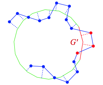
To compute accuracy, for each vertex on R, we find the nearest point on G. We augment G with a hole filled region (solid red) to give a mesh G'. Vertices (shown in red) that project to the hole filled region are not used in the accuracy metric.