Results
Table of Content
Evaluation questions
Given a specific description, the proof-of-concept interpreter will select an algorithm, and any object that matches this description should be well reconstructed by this algorithm. We use the descriptions that match the problem conditions of the testing objects so that each object should at least return one well reconstructed result. Since a problem condition could be mapped to multiple algorithms, an object that doesn’t match the description could potentially have a satisfactory result as well.
Datasets
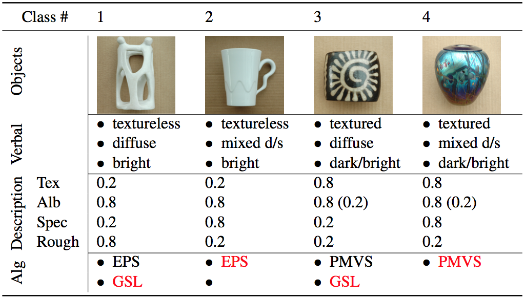
We generate a dataset of four objects, see Dataset and Recon page. The mapping from problem conditions to algorithms are summarized in the table below. The reconstruction results of test objects and those of the baseline method are shown in the Figure 1. See the corresponding videos for mor details.
| Class # | Object | Texture | Albedo | Specular | Rough | Mapping |
|---|---|---|---|---|---|---|
| 1 | barrel | 0.8 | 0.8 | 0.2 | 0.8 | PMVS, EPS, GSL |
| 2 | vase0 | 0.8 | 0.8 | 0.8 | 0.2 | PMVS, EPS |
| 3 | bust | 0.2 | 0.8 | 0.2 | 0.8 | EPS, GSL |
| 4 | vase1 | 0.2 | 0.8 | 0.8 | 0.2 | EPS |
We generate a real-world dataset, see page Dataset and Recon. The mapping from problem conditions to algorithms are summarized in the table below.
| Class # | Object | Texture | Albedo | Specular | Rough | Mapping |
|---|---|---|---|---|---|---|
| 1 | pot | 0.8 | 0.8(0.2) | 0.2 | 0.8 | PMVS, GSL |
| 2 | vase | 0.8 | 0.5(0.2) | 0.5 | 0.2 | PMVS |
| 3 | status | 0.2 | 0.8 | 0.2 | 0.8 | EPS, GSL |
| 4 | cup | 0.2 | 0.8 | 0.5 | 0.2 | EPS, GSL |

Synthetic data
Real-world data
Evaluation 1: accurate description, successful result
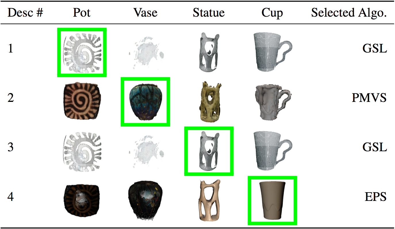
In this section, we evaluate whether the interpreter can return a successful reconstruction result given a valid description of problem condition, see results in Figure 2. The figure is divided into two sections, one for synthetic dataset and another for real-world dataset. The ‘Algo’ row shows the algorithm selected by the interpreter. The ‘Results’ row shows the reconstruction results of the corresponding algorithm, and the ‘Baseline’ row demonstrate the results of the baseline method. We utilize visual phenomena, such as surface roughness, holes, spikes as indicators of the reconstruction quality.
The baseline method achieves decent reconstruction results on all objects. Though due to the resolution of the voxel grids, the surfaces are relatively rough. Further, the surface concavities fail to be carved out for concave objects (Bust). The performance of the interpreter on both synthetic and real-world datasets are consistent in that the algorithms selected by the interpreter consistently outperform the baseline technique. All results have much smoother reconstructed surfaces, especially those of EPS and GSL, which is an indicator that the accuracy of the results are much higher using the selected algorithm. Further, erroneous results, such as surface holes, obtrutions, spikes are absent from the reconstruction results, which indi- cates that the selected algorithms can achieve completeness, and angular error no worse than the baseline.
Note that the selection of objects do no favor any algorithm. In fact, as we will show below, it is highly possible to get a poor result if another algorithm is chosen instead of the interpreted one. The significance of this study is that we demonstrated that it is achievable to translate a user-specified description, which has nothing to do with algorithm-level knowledge, to an algorithm selected from a suite of algorithms and achieve a successful reconstruction. There is no need to understand the underlying algorithms, or set the obscure algorithm specific parameters.

Synthetic data

Real-world data
Evaluation 2: less accurate description, less successful results
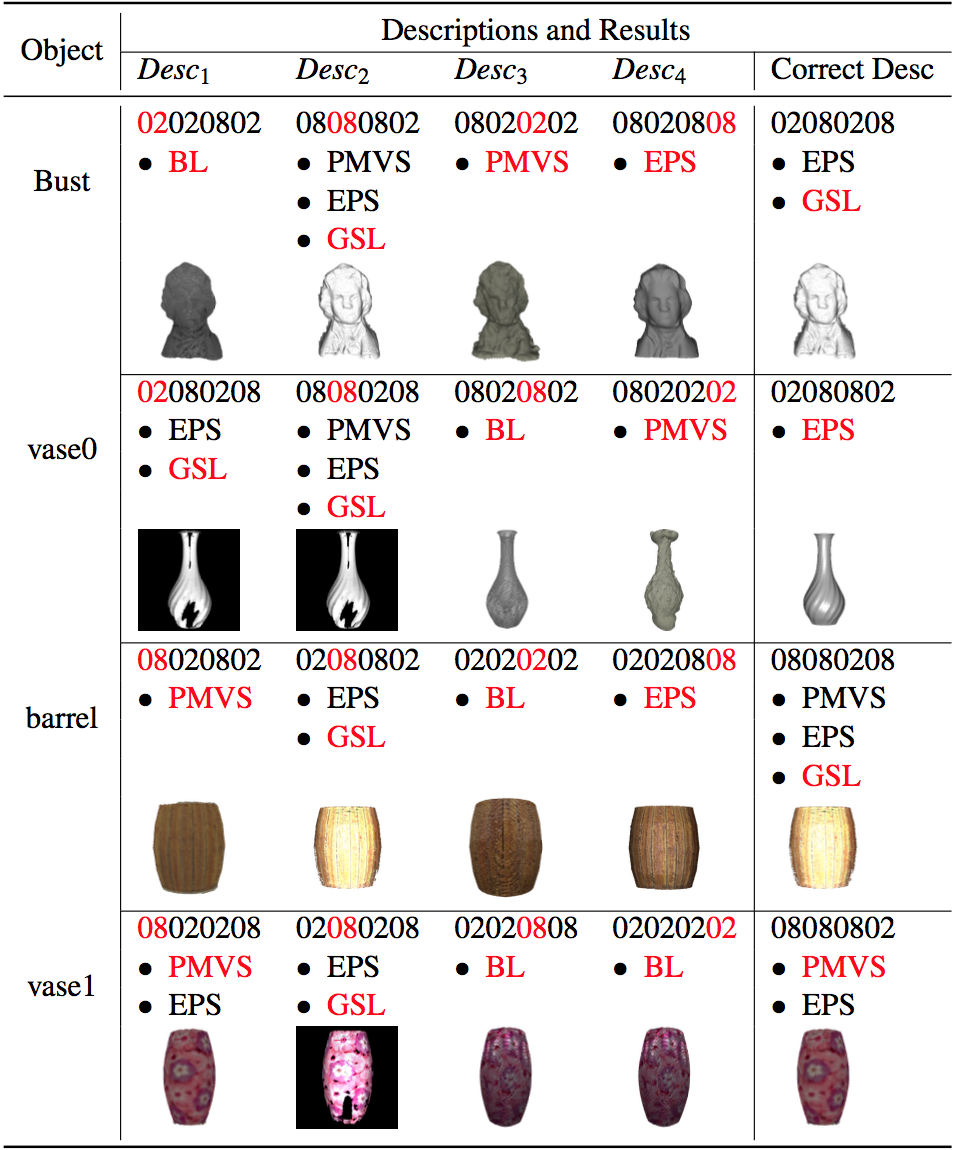
We have demonstrated in last section that the interpreter can achieve successful results given accurate description. However, how would the interpreter perform given an inaccurate description? There are two guesses: 1) the interpreter would return poor result given an inaccurate description; 2) the interpreter can still achieve successful results under some specific circumstances. In this section, we are inter- ested to find out how sensitive the interpreter is given inaccurate descriptions, and the cases where it would fail or succeed. We provide four inaccurate desriptions by iterating through four properties, and each time one and only one property is set correctly. For instance, propi is correctly estimated for desci while the rest of the properties are set incorrectly, . Since a description could be mapped to multiple algorithms, a description that does not match the object could potentially have a successful reconstruction result as well.
The layout of the graph is as follows: columnwise, presents results where an inaccurate description is provided while the last column presents the results where the correct description is provided. Rowwise, for each object, the result is divided into three segments: The description of problem condition is presented in the first segment, which is coloured-coded to indicate the correctly set property. The order of properties in the description is: texture, albedo, specularity, and roughness. Since there is one and only one correctly estimated property in each inaccurate description, it is coloured in red while the incorrectly estimated properties are coloured in black. The algorithms returned by the mapping are presented below the description in the second segment, with the algorithm chosen by the interpreter coloured in red. The reconstruction result using the interpreted algorithm is shown in the last segment of each section. Let’s denote the algorithm(s) returned by the mapping given description Desci as . For instance, the algorithms for object bust given description Desc2 is . Let’s also denote the algorithm(s) returned by the correct description as . Thus in the case of object bust, . We observe that an inaccurate description can possibly lead to a successful reconstruction if and only if
The reason is that there are multiple algorithms that could work successfully for a specific object. Thus if an algorithm other than the interpreted one is chosen given an inaccurate description, a successful reconstruction result is still achievable. Let’s use bust as an example, and lead to poor results whereas and result in successful reconstructions. We can see that neither nor is mapped to any algorithm that is in common with those returned given accurate description. Further, both and have at least one mapped algorithm that coincides with the algorithms returned given accurate description. The take-away message is that for an incorrect description, the reconstruction results are generally worse than that of the interpreted result. However, for conditions that have multiple working algorithms, there may very well be an acceptable result.
Synthetic data

Real-world data
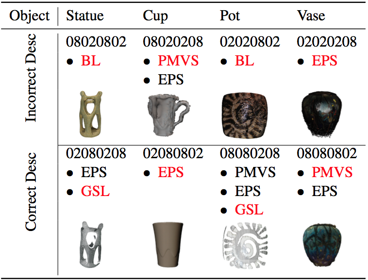
Evaluation 3: inaccurate description, poor reconstruction results
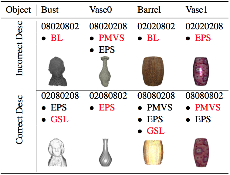
We have demonstrated that given a less accurate description, the results may or may not be poor. In cases where the algorithms mapped from inaccurate description coincide with algorithms returned from accurate description, it is still possible to achieve successful reconstruction. In this section, we are interested to see if this conclusion can also be applied to complete inaccurate description, i.e., is it still possible to return a successful result. In this section, we evaluate whether the interpreter would return a poor reconstruction result given an inaccurate description of problem condition. We evaluate the performance of the interpreter using both synthetic and real-world objects.
The figure is divided into two sections: one for inaccurate description and one for accurate description. The inaccurate description is property-wise opposite to the corresponding accurate description. The mapped algorithms are shown below the description, with the algorithm chosen by the interpreter coloured in red. The reconstruction result by the interpreted algorithm is shown as well.
From the study of less accurate desription, we have already found out that it is still possible to achieve a successful result given an inaccurate description. However, it becomes more challenging, and more likely to select a less successful algorithm or the baseline method. There is a certain limit to the tolerance of inaccuracy of property estimation. Thus, the take-away message is that the interpreter, in some cases, can still performs reliably given an inaccurate description. However, it becomes more likely to fail to achieve a successful result given an completely inaccurate description of problem condition.
Synthetic data
Real-world data
Summary
This chapter, we proposed a proof of concept interpreter, and provide demonstrative results of the performance of the interpreter. We are interested to see if the interpreter is able to handle conditions where accurate or inaccurate descriptions are provided. The findings can be further summarized into one graph, as shown in Figure 5.

Synthetic data